I. About the data set
I obtained this data set from Kaggle1, and Sakshi Goyal uploaded it in 2020. This data set is about a 🏦bank’s customer churn issue. The manager💼 of the bank is interested in predicting which customer will leave this bank💸. By doing so, the bank can target those customers with special products and services to increase their satisfaction and customer retention🌞.
It contains 10,127 observations and 23 variables. Because I had some issues with Income Category values, so I add another column that used a scale of 1 through 5 to represent each income category in Excel before importing it to the Rstudio. My data analyses are based on 20 variables, which excluded the Client Number and two Naive Bayes Classifiers😶.
The purpose of this project is to predict churned customers, so I use recall as an important model fit measurement📐. I also include accuracy and kappa as measurements of model fitness. I choose kappa because customer churn is only around 16% of total customers. Although some studies state kappa is not a good measure for classification model2, I think it is good enough for this project😎 I include a comparison table📊 in the last section, Result for each models’ performance.
II. Descriptive Stats
This data set has 9,664 missing values, which is 4.77% of the 202,540 total values. Most of those missing values are belong to categorical variables.
After using kNN to replace all the missing data by calculating their nearest 10 neighbors 🏠🏡 values, the new data set contains 0️⃣ missing values. The distribution of the target variable is not balanced⚖️, as attrited customers only represent 16% of the total customers. Because of the potential overfitting issue, I used caret’s built-in function SMOTE oversampling to overcome this issue, and it did improved the model performance. Below are some visualizations that are used for gaining some insights of the underlying data.
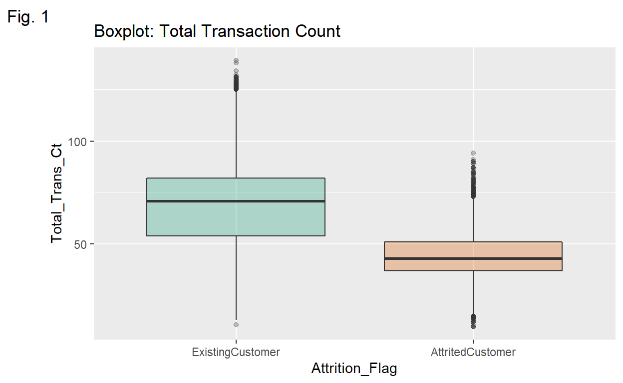
Transaction Count Attrited customer group has less variability and less spread regarding the total number of transactions. We can see that 50% of customer churns have less than 50 transaction counts and no of those customers have more than 100 transactions.
Show code
ggplot(data = BankChurners1,
       mapping = aes(x = Attrition_Flag,
                     y = Total_Trans_Ct,
                     fill = Attrition_Flag)) +
  labs(title = "Boxplot: Total Transaction Count",
       tag = "Fig. 1") +
  geom_boxplot(alpha = .3) +
  theme(legend.position = "none") +
  scale_fill_brewer(palette = "Dark2")
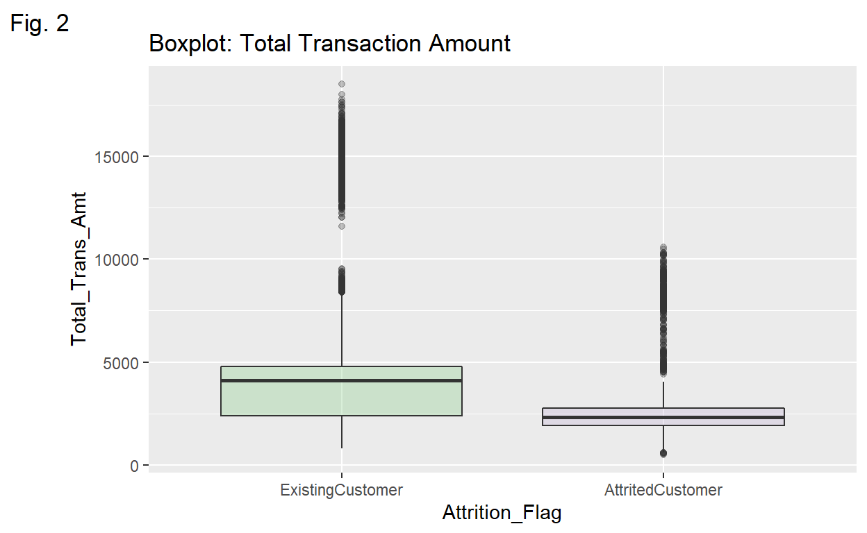
Transaction Amt💵 Both existing and attrited Customers are right-skewed due to outliers regarding their total transaction amounts.
Show code
ggplot(data = BankChurners1,
       mapping = aes(x = Attrition_Flag,
                     y = Total_Trans_Amt,
                     fill = Attrition_Flag)) +
  labs(title = "Boxplot: Total Transaction Amount",
       tag = "Fig. 2") +
  geom_boxplot(alpha = .3) +
  theme(legend.position = "none") +
  scale_fill_brewer(palette = "Accent")
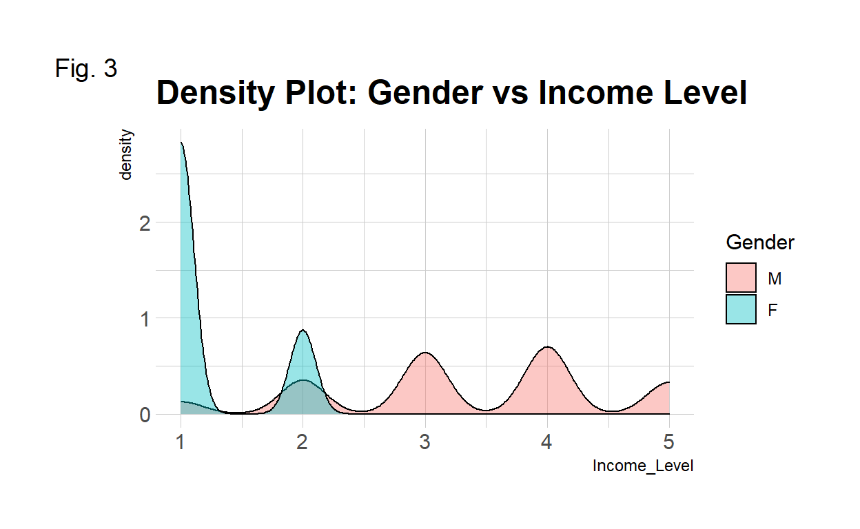
🌠Credit Limit The majority of attrited customers have lower than $5000 credit.
Show code
ggplot(data = BankChurners1,
       mapping = aes(x = Credit_Limit,
                     fill = Attrition_Flag)) +
  geom_histogram(color = "#e9ecef",
                 alpha = 1,
                 position = "stack") +
  scale_fill_manual(values=c("#adb8ff", "#e8b5ff")) +
  theme_ipsum() +
  labs(title = "Histogram: Credit Limit vs Attrition",
       tag = "Fig. 4")
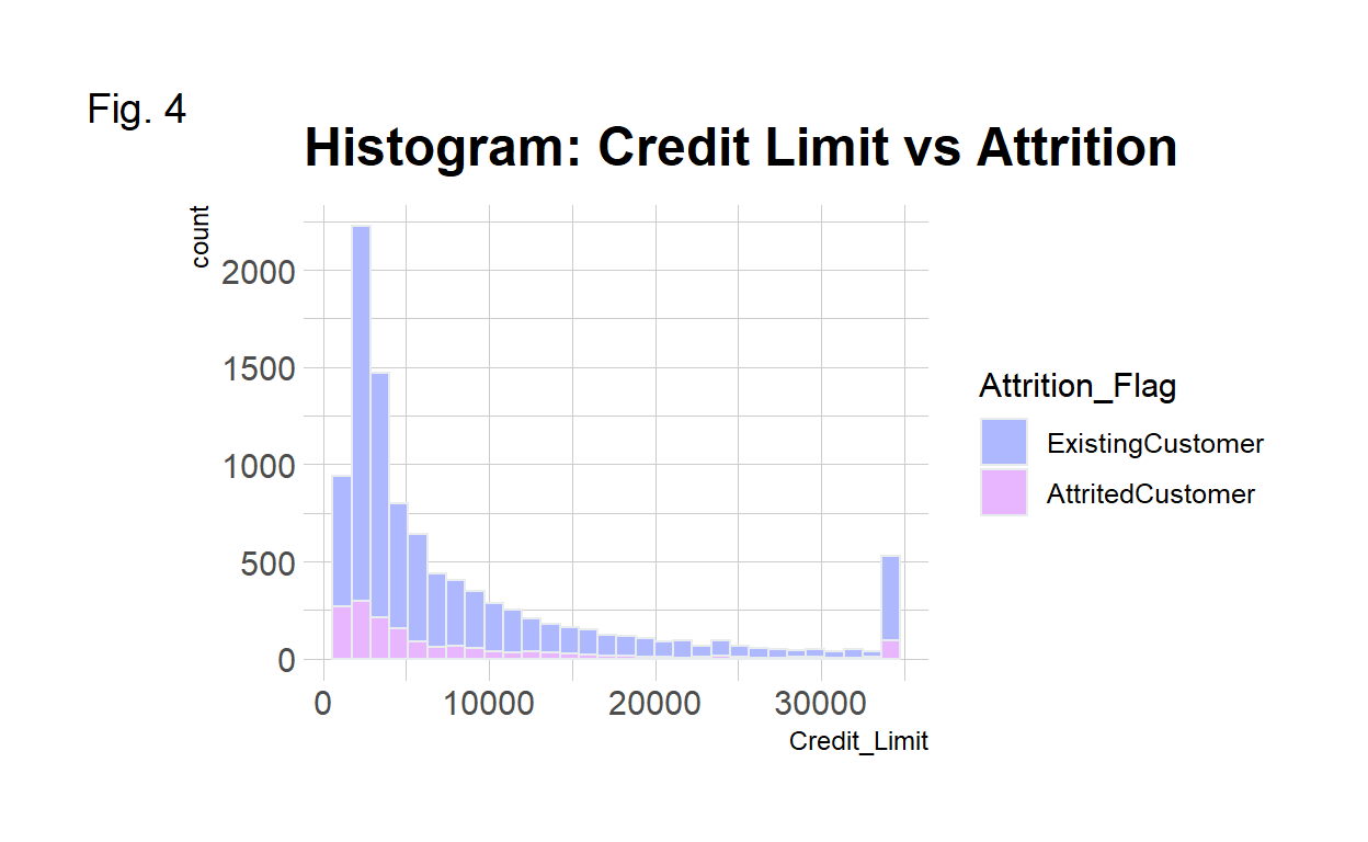
Income vs Gender Females’ income levels are concentrated at low levels such as levels 1 and 2 while males have much higher income level distributions.
Show code
ggplot(data = BankChurners1,
       mapping = aes(x = Income_Level,
                     group = Gender,
                     fill = Gender)) +
  geom_density(adjust = 1.5, alpha = .4) +
  theme_ipsum() +
  labs(title = "Density Plot: Gender vs Income Level",
       tag = "Fig. 3") +
  scale_color_manual(values=c("M"="blue", "F"="pink")) # not working
III. The Models
The three models used for this project are as follow:
- Random Forest🌳: Decision trees are sensitive to changes, introducing randomness to each split of trees, reduces the over-fitting issue. Also, random forest uses bagging method to make decisions based on a majority vote from each individual tree.
- Gradient Boosting Tree🌲: Gradient boosting is normally better💪 than random forest due to its arbitrary cost functions for classification purpose3.
- Neural Network🔮: Neural network is very effective and efficient in making inferences and detecting patterns from complex data sets. It uses the input information to optimize the weight of those inputs and then generates outputs. It also minimizes the errors ❌ of those outputs to improve those processed inputs until the errors become small enough🔄. The final result is based on minimized errors❓
IV. The Process
I split the data set into the training set and testing set based on 4 different ratios, and the 7:3 ratio has the best result, so I use this ratio for rest of models: 🌳random forest, gradient boosting tree🌲, and 💫neural network🔮 to train🚋 each data set. After importing the original data set, I use the kNN function with k = 10 to replace those missing values. For comparison, I replace missing values only in the training set and leave the testing set as it is. Both random forest and gradient boosting trees have better performance in terms of recall after re-sampling in the training sets. Neural network model turns out to have the worst performance. I am going to use SOMTE for the neural network model just to see the comparison. It does improved the recall quit bit even though the accuracy decreased a bit. I will update the comparsion table and the result description late.
V. Code
i. 🎄Random Forest Total NA⭐
Original data set with Total Missing Value Replaced
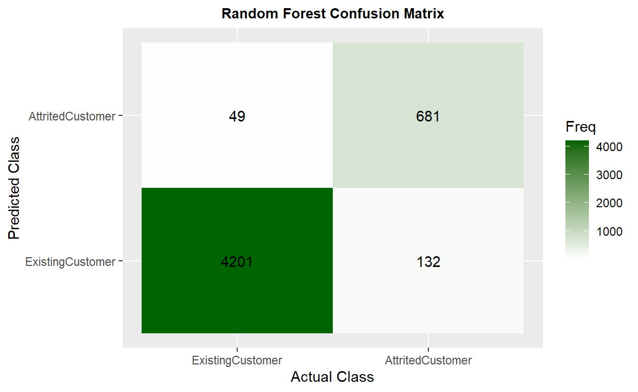
I use 4 different ratio to split the data set into a training set and a testing set. The 7:3 ratio has the best performance. The model has 0.9661 of accuracy🎯 and 0.8683 in kappa, this huge drop probably is due to the imbalanced distribution of the attrition. The recall is 0.8381, which means that this model will misclassify 2 attrited customers of every 10 customers as existing customers.
Show code
comparison <- matrix(c(0.9599, 0.8437, 0.8155, 0.9590, 0.8406, 0.8154, 0.9661, 0.8683, 0.8381, 0.9580, 0.8359, 0.8062),
                    ncol = 3, byrow = TRUE)
colnames(comparison) <- c("Accuracy", "Kappa", "Recall")
rownames(comparison) <- c("5:5", "6:4", "7:3", "8:2")
comparison <- as.data.frame.matrix(comparison)
kable(comparison) %>%
  row_spec(3, color = "white", background = "#bdaeea")
| Accuracy | Kappa | Recall | |
|---|---|---|---|
| 5:5 | 0.9599 | 0.8437 | 0.8155 |
| 6:4 | 0.9590 | 0.8406 | 0.8154 |
| 7:3 | 0.9661 | 0.8683 | 0.8381 |
| 8:2 | 0.9580 | 0.8359 | 0.8062 |
5:5 Data split in 5:5 ratio.
Show code
# data split
index <- createDataPartition(BankChurners2$Attrition_Flag,
                             p = .5, list = FALSE, times = 1)
train <- BankChurners2[index,]
test <- BankChurners2[-index,]

# train1
churn_RF1 <- train(
  form = factor(Attrition_Flag) ~.,
  data = train,
  trControl = trainControl(method = "cv",
                           number = 10,
                           classProbs = TRUE),
  method = "rf",
  tuneLength = 10
)
# churn_RF1

# feature importance
var_imp1 <- varImp(churn_RF1)$importance %>%
  arrange(desc(Overall))
kable(head(var_imp1))
| Overall | |
|---|---|
| Total_Trans_Amt | 100.00000 |
| Total_Trans_Ct | 93.11644 |
| Total_Ct_Chng_Q4_Q1 | 63.25446 |
| Total_Relationship_Count | 41.57094 |
| Total_Amt_Chng_Q4_Q1 | 36.03208 |
| Total_Revolving_Bal | 32.73355 |
Show code
ggplot(var_imp1, aes(x = reorder(rownames(var_imp1), Overall), y = Overall)) +
  geom_point(color = "plum1", size = 6, alpha = 1) +
  geom_segment(aes(x = rownames(var_imp1), xend = rownames(var_imp1),
                   y = 0, yend = Overall), color = "skyblue") +
  xlab("Variable") +
  ylab("Overall Importance") +
  theme_light() +
  coord_flip()

Show code
# test1
churn_RF_pred1 <- predict(churn_RF1, test, type = "prob")
churn_RF_test_pred1 <- cbind(churn_RF_pred1, test)
churn_RF_test_pred1 <- churn_RF_test_pred1 %>%
  mutate(prediction = if_else(AttritedCustomer > ExistingCustomer,
                              "AttritedCustomer", "ExistingCustomer"))
table(churn_RF_test_pred1$prediction)
AttritedCustomer ExistingCustomer
             730             4333
Show code
# result1
churn_matrix1 <- confusionMatrix(factor(churn_RF_test_pred1$prediction),
                                 factor(churn_RF_test_pred1$Attrition_Flag),
                                 positive = "AttritedCustomer")
churn_matrix1
Confusion Matrix and Statistics

                  Reference
Prediction         ExistingCustomer AttritedCustomer
  ExistingCustomer             4201              132
  AttritedCustomer               49              681

               Accuracy : 0.9643
                 95% CI : (0.9588, 0.9692)
    No Information Rate : 0.8394
    P-Value [Acc > NIR] : < 2.2e-16

                  Kappa : 0.8617

 Mcnemar's Test P-Value : 1.094e-09

            Sensitivity : 0.8376
            Specificity : 0.9885
         Pos Pred Value : 0.9329
         Neg Pred Value : 0.9695
             Prevalence : 0.1606
         Detection Rate : 0.1345
   Detection Prevalence : 0.1442
      Balanced Accuracy : 0.9131

       'Positive' Class : AttritedCustomer
Show code
# Accuracy : 0.9632  Kappa : 0.8586 Sensitivity : 0.8431

ggplot(as.data.frame(churn_matrix1$table)) +
  geom_raster(aes(x = Reference, y = Prediction, fill = Freq)) +
  geom_text(aes(x = Reference, y = Prediction, label = Freq)) +
  scale_fill_gradient2(low = "darkred", high = "darkgreen",
                       na.value = "gray", name = "Freq") +
  scale_x_discrete(name = "Actual Class") +
  scale_y_discrete(name = "Predicted Class") +
  ggtitle("Random Forest Confusion Matrix") +
  theme(plot.title = element_text(hjust = .5, size = 10, face = "bold"))
6:4 Data split in 6:4 ratio.
Show code
# data split
index <- createDataPartition(BankChurners2$Attrition_Flag,
                             p = .6, list = FALSE, times = 1)
train <- BankChurners2[index,]
test <- BankChurners2[-index,]

# train1
churn_RF1 <- train(
  form = factor(Attrition_Flag) ~.,
  data = train,
  trControl = trainControl(method = "cv",
                           number = 10,
                           classProbs = TRUE),
  method = "rf",
  tuneLength = 10
)
# churn_RF1

# test1
churn_RF_pred1 <- predict(churn_RF1, test, type = "prob")
churn_RF_test_pred1 <- cbind(churn_RF_pred1, test)
churn_RF_test_pred1 <- churn_RF_test_pred1 %>%
  mutate(prediction = if_else(AttritedCustomer > ExistingCustomer,
                              "AttritedCustomer", "ExistingCustomer"))

# result1
churn_matrix1 <- confusionMatrix(factor(churn_RF_test_pred1$prediction),
                                 factor(churn_RF_test_pred1$Attrition_Flag),
                                 positive = "AttritedCustomer")
churn_matrix1
Confusion Matrix and Statistics

                  Reference
Prediction         ExistingCustomer AttritedCustomer
  ExistingCustomer             3354              117
  AttritedCustomer               46              533

               Accuracy : 0.9598
                 95% CI : (0.9532, 0.9656)
    No Information Rate : 0.8395
    P-Value [Acc > NIR] : < 2.2e-16

                  Kappa : 0.8437

 Mcnemar's Test P-Value : 4.186e-08

            Sensitivity : 0.8200
            Specificity : 0.9865
         Pos Pred Value : 0.9206
         Neg Pred Value : 0.9663
             Prevalence : 0.1605
         Detection Rate : 0.1316
   Detection Prevalence : 0.1430
      Balanced Accuracy : 0.9032

       'Positive' Class : AttritedCustomer
Show code
# Accuracy : 0.9632 Kappa : 0.8586 Sensitivity : 0.8431
7:3 Data split in 7:3 ratio.
Show code
# data split
index <- createDataPartition(BankChurners2$Attrition_Flag,
                             p = .7, list = FALSE, times = 1)
train <- BankChurners2[index,]
test <- BankChurners2[-index,]

# train1
churn_RF1 <- train(
  form = factor(Attrition_Flag) ~.,
  data = train,
  trControl = trainControl(method = "cv",
                           number = 10,
                           classProbs = TRUE),
  method = "rf",
  tuneLength = 10
)
# churn_RF1

# test1
churn_RF_pred1 <- predict(churn_RF1, test, type = "prob")
churn_RF_test_pred1 <- cbind(churn_RF_pred1, test)
churn_RF_test_pred1 <- churn_RF_test_pred1 %>%
  mutate(prediction = if_else(AttritedCustomer > ExistingCustomer,
                              "AttritedCustomer", "ExistingCustomer"))
table(churn_RF_test_pred1$prediction)
AttritedCustomer ExistingCustomer
             444             2594
Show code
# result1
churn_matrix1 <- confusionMatrix(factor(churn_RF_test_pred1$prediction),
                                 factor(churn_RF_test_pred1$Attrition_Flag),
                                 positive = "AttritedCustomer")
churn_matrix1
Confusion Matrix and Statistics

                  Reference
Prediction         ExistingCustomer AttritedCustomer
  ExistingCustomer             2519               75
  AttritedCustomer               31              413

               Accuracy : 0.9651
                 95% CI : (0.958, 0.9713)
    No Information Rate : 0.8394
    P-Value [Acc > NIR] : < 2.2e-16

                  Kappa : 0.8657

 Mcnemar's Test P-Value : 2.96e-05

            Sensitivity : 0.8463
            Specificity : 0.9878
         Pos Pred Value : 0.9302
         Neg Pred Value : 0.9711
             Prevalence : 0.1606
         Detection Rate : 0.1359
   Detection Prevalence : 0.1461
      Balanced Accuracy : 0.9171

       'Positive' Class : AttritedCustomer
8:2 Data split in 8:2 ratio.
Show code
# data split
index <- createDataPartition(BankChurners2$Attrition_Flag,
                             p = .8, list = FALSE, times = 1)
train <- BankChurners2[index,]
test <- BankChurners2[-index,]

# train1
churn_RF1 <- train(
  form = factor(Attrition_Flag) ~.,
  data = train,
  trControl = trainControl(method = "cv",
                           number = 10,
                           classProbs = TRUE),
  method = "rf",
  tuneLength = 10
)

# test1
churn_RF_pred1 <- predict(churn_RF1, test, type = "prob")
churn_RF_test_pred1 <- cbind(churn_RF_pred1, test)
churn_RF_test_pred1 <- churn_RF_test_pred1 %>%
  mutate(prediction = if_else(AttritedCustomer > ExistingCustomer,
                              "AttritedCustomer", "ExistingCustomer"))

# result1
churn_matrix1 <- confusionMatrix(factor(churn_RF_test_pred1$prediction),
                                 factor(churn_RF_test_pred1$Attrition_Flag),
                                 positive = "AttritedCustomer")
churn_matrix1
Confusion Matrix and Statistics

                  Reference
Prediction         ExistingCustomer AttritedCustomer
  ExistingCustomer             1683               41
  AttritedCustomer               17              284

               Accuracy : 0.9714
                 95% CI : (0.9631, 0.9782)
    No Information Rate : 0.8395
    P-Value [Acc > NIR] : < 2.2e-16

                  Kappa : 0.8904

 Mcnemar's Test P-Value : 0.002527

            Sensitivity : 0.8738
            Specificity : 0.9900
         Pos Pred Value : 0.9435
         Neg Pred Value : 0.9762
             Prevalence : 0.1605
         Detection Rate : 0.1402
   Detection Prevalence : 0.1486
      Balanced Accuracy : 0.9319

       'Positive' Class : AttritedCustomer
ii. 🌴Random Forest NA & Var🍃
data set with 14 variables and Total Missing Value Replaced
Education level🎓, marital status💑, card category💳, income level💰, dependent count👶, and gender👦 👩 are the least important variables that used for the final prediction. After dropping those 6 variables, the model performance decreased a little bit compared to the previous model’s.
Show code
# data split drop 6 var
BankChurners_drop_var <- BankChurners2[-c(3:8)]
index_var <- createDataPartition(BankChurners_drop_var$Attrition_Flag,
                                 p = .7, list = FALSE, times = 1)
train_var <- BankChurners_drop_var[index,]
test_var <- BankChurners_drop_var[-index,]

# train drop 6 var
churn_RF_var <- train(
  form = factor(Attrition_Flag) ~.,
  data = train_var,
  trControl = trainControl(method = "cv",
                           number = 10,
                           classProbs = TRUE),
  method = "rf",
  tuneLength = 10
)
# churn_RF_var

# test drop 6 var
churn_RF_pred_var <- predict(churn_RF_var, test_var, type = "prob")
churn_RF_test_pred_var <- cbind(churn_RF_pred_var, test_var)
churn_RF_test_pred_var <- churn_RF_test_pred_var %>%
  mutate(prediction = if_else(AttritedCustomer > ExistingCustomer,
                              "AttritedCustomer", "ExistingCustomer"))
table(churn_RF_test_pred_var$prediction)
AttritedCustomer ExistingCustomer
             299             1726
Show code
# result drop 6 var
churn_matrix_var <- confusionMatrix(factor(churn_RF_test_pred_var$prediction),
                                    factor(churn_RF_test_pred_var$Attrition_Flag),
                                    positive = "AttritedCustomer")
churn_matrix_var
Confusion Matrix and Statistics

                  Reference
Prediction         ExistingCustomer AttritedCustomer
  ExistingCustomer             1682               44
  AttritedCustomer               18              281

               Accuracy : 0.9694
                 95% CI : (0.9609, 0.9764)
    No Information Rate : 0.8395
    P-Value [Acc > NIR] : < 2.2e-16

                  Kappa : 0.8826

 Mcnemar's Test P-Value : 0.001498

            Sensitivity : 0.8646
            Specificity : 0.9894
         Pos Pred Value : 0.9398
         Neg Pred Value : 0.9745
             Prevalence : 0.1605
         Detection Rate : 0.1388
   Detection Prevalence : 0.1477
      Balanced Accuracy : 0.9270

       'Positive' Class : AttritedCustomer
iii. Random Forest Train NA✨
Original data set with Training Set Missing Value Replaced
Only replaced missing values in the training set. The model has 0.9575 in accuracy and 0.8341 in kappa, which improved 📈 compared to the previous model. The recall is 0.8062, which means that this model will misclassify 1 attrited customer of every 10 customers as existing customers.
Show code
# data split
index2 <- createDataPartition(BankChurners1$Attrition_Flag,
                              p = .7, list = FALSE, times = 1)
train2 <- BankChurners1[index,]
test2 <- BankChurners1[-index,]
table(is.na(train2))
 FALSE   TRUE
154354   7686
Show code
# replace missing values in the training set
train2 <- VIM::kNN(train2,
                   variable = c("Dependent_count", "Education_Level",
                                "Marital_Status", "Income_Level",
                                "Months_Inactive_12_mon", "Contacts_Count_12_mon",
                                "Total_Revolving_Bal", "Total_Amt_Chng_Q4_Q1",
                                "Total_Ct_Chng_Q4_Q1", "Avg_Utilization_Ratio"),
                   k = 10)
# summary(train2)
train2 <- train2[, -c(21:30)]
table(is.na(train2))
 FALSE
162040
Show code
# train2
churn_RF2 <- train(
  form = factor(Attrition_Flag) ~.,
  data = train2,
  trControl = trainControl(method = "cv",
                           number = 10,
                           classProbs = TRUE),
  method = "rf",
  tuneLength = 10
)
# churn_RF2

# test1
churn_RF_pred2 <- predict(churn_RF2, test, type = "prob")
churn_RF_test_pred2 <- cbind(churn_RF_pred2, test)
churn_RF_test_pred2 <- churn_RF_test_pred2 %>%
  mutate(prediction = if_else(AttritedCustomer > ExistingCustomer,
                              "AttritedCustomer", "ExistingCustomer"))
table(churn_RF_test_pred2$prediction)
AttritedCustomer ExistingCustomer
             301             1724
Show code
#result1
churn_matrix2 <- confusionMatrix(factor(churn_RF_test_pred2$prediction),
                                 factor(churn_RF_test_pred2$Attrition_Flag),
                                 positive = "AttritedCustomer")
churn_matrix2
Confusion Matrix and Statistics

                  Reference
Prediction         ExistingCustomer AttritedCustomer
  ExistingCustomer             1682               42
  AttritedCustomer               18              283

               Accuracy : 0.9704
                 95% CI : (0.962, 0.9773)
    No Information Rate : 0.8395
    P-Value [Acc > NIR] : < 2.2e-16

                  Kappa : 0.8867

 Mcnemar's Test P-Value : 0.002985

            Sensitivity : 0.8708
            Specificity : 0.9894
         Pos Pred Value : 0.9402
         Neg Pred Value : 0.9756
             Prevalence : 0.1605
         Detection Rate : 0.1398
   Detection Prevalence : 0.1486
      Balanced Accuracy : 0.9301

       'Positive' Class : AttritedCustomer
Show code
ggplot(as.data.frame(churn_matrix2$table)) +
  geom_raster(aes(x = Reference, y = Prediction, fill = Freq)) +
  geom_text(aes(x = Reference, y = Prediction, label = Freq)) +
  scale_fill_gradient2(low = "darkred", high = "plum1",
                       na.value = "gray", name = "Freq") +
  scale_x_discrete(name = "Actual Class") +
  scale_y_discrete(name = "Predicted Class") +
  ggtitle("Random Forest Confusion Matrix") +
  theme(plot.title = element_text(hjust = .5, size = 10, face = "bold"))

iv. Random Forest Total NA & SMOTE❄️
Original data set with Total Missing Value Replaced and Resampling in the Training Set
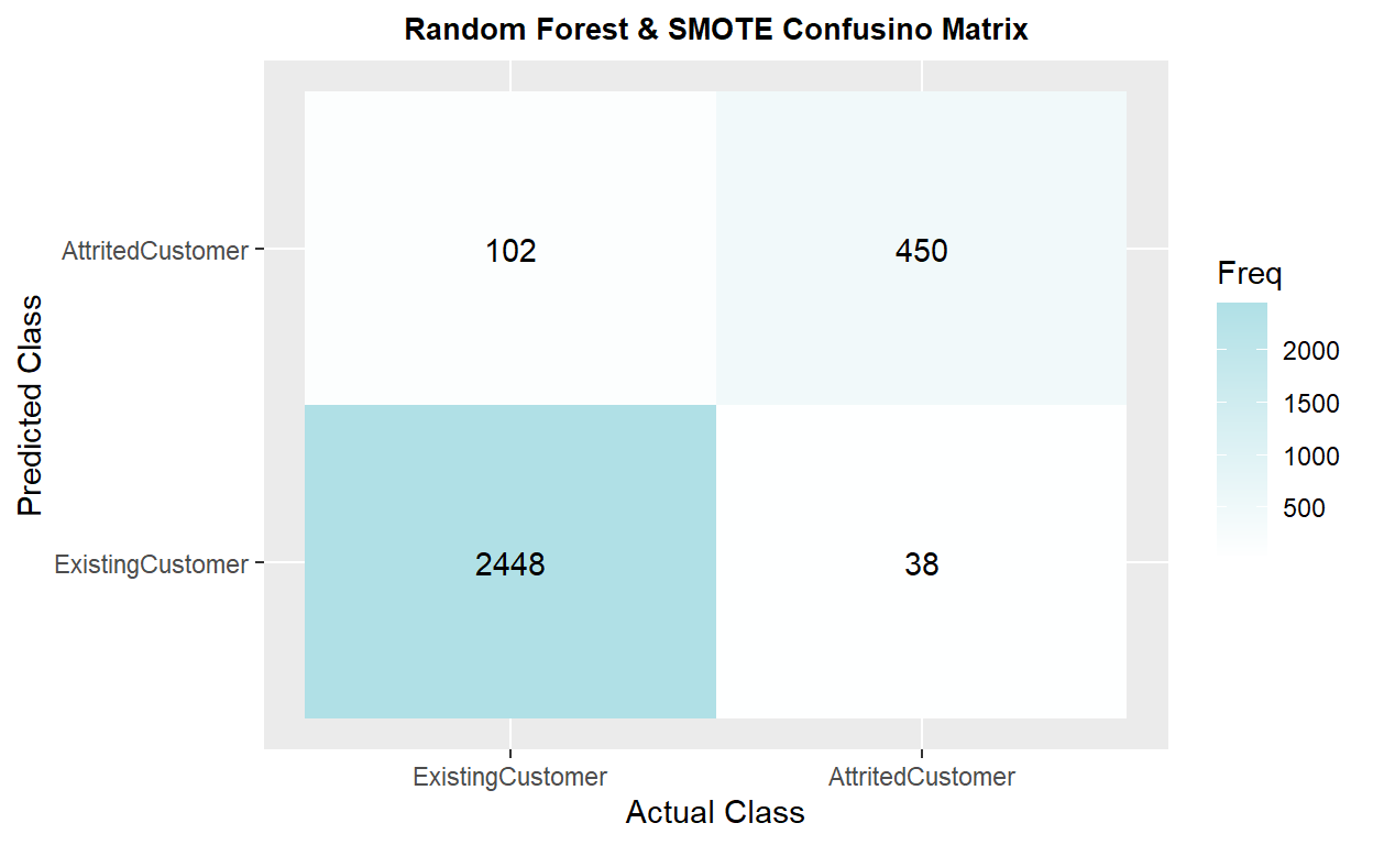
The model has 0.9549 of accuracy and 0.8423 in kappa, which is similar to the previous model. The recall is 0.9344, the highest score among other models.
Show code
# data split
index <- createDataPartition(BankChurners2$Attrition_Flag,
                             p = .7, list = FALSE, times = 1)
train <- BankChurners2[index,]
test <- BankChurners2[-index,]

# train3
churn_RF3 <- train(
  form = factor(Attrition_Flag) ~.,
  data = train,
  trControl = trainControl(method = "cv",
                           number = 10,
                           classProbs = TRUE,
                           sampling = "smote"),
  method = "rf",
  tuneLength = 10
)
# churn_RF3

# feature importance
var_imp3 <- varImp(churn_RF3)$importance %>%
  arrange(desc(Overall))
kable(head(var_imp3))
| Overall | |
|---|---|
| Total_Trans_Ct | 100.00000 |
| Total_Trans_Amt | 71.55841 |
| Total_Ct_Chng_Q4_Q1 | 35.62309 |
| Total_Relationship_Count | 26.05581 |
| Months_Inactive_12_mon | 19.63056 |
| Total_Amt_Chng_Q4_Q1 | 14.54063 |
Show code
ggplot(var_imp3, aes(x = reorder(rownames(var_imp3), Overall), y = Overall)) +
  geom_point(color = "plum1", size = 6, alpha = 1) +
  geom_segment(aes(x = rownames(var_imp3), xend = rownames(var_imp3),
                   y = 0, yend = Overall), color = "skyblue") +
  xlab("Variable") +
  ylab("Overall Importance") +
  theme_light() +
  coord_flip()

Show code
# test3
churn_RF_pred3 <- predict(churn_RF3, test, type = "prob")
churn_RF_test_pred3 <- cbind(churn_RF_pred3, test)
churn_RF_test_pred3 <- churn_RF_test_pred3 %>%
  mutate(prediction = if_else(AttritedCustomer > ExistingCustomer,
                              "AttritedCustomer", "ExistingCustomer"))
table(churn_RF_test_pred3$prediction)
AttritedCustomer ExistingCustomer
             552             2486
Show code
# result3
churn_matrix3 <- confusionMatrix(factor(churn_RF_test_pred3$prediction),
                                 factor(churn_RF_test_pred3$Attrition_Flag),
                                 positive = "AttritedCustomer")
churn_matrix3
Confusion Matrix and Statistics

                  Reference
Prediction         ExistingCustomer AttritedCustomer
  ExistingCustomer             2448               38
  AttritedCustomer              102              450

               Accuracy : 0.9539
                 95% CI : (0.9458, 0.9611)
    No Information Rate : 0.8394
    P-Value [Acc > NIR] : < 2.2e-16

                  Kappa : 0.8377

 Mcnemar's Test P-Value : 1.012e-07

            Sensitivity : 0.9221
            Specificity : 0.9600
         Pos Pred Value : 0.8152
         Neg Pred Value : 0.9847
             Prevalence : 0.1606
         Detection Rate : 0.1481
   Detection Prevalence : 0.1817
      Balanced Accuracy : 0.9411

       'Positive' Class : AttritedCustomer
Show code
ggplot(as.data.frame(churn_matrix3$table)) +
  geom_raster(aes(x = Reference, y = Prediction, fill = Freq)) +
  geom_text(aes(x = Reference, y = Prediction, label = Freq)) +
  scale_fill_gradient2(low = "darkred", high = "powderblue",
                       na.value = "gray", name = "Freq") +
  scale_x_discrete(name = "Actual Class") +
  scale_y_discrete(name = "Predicted Class") +
  ggtitle("Random Forest & SMOTE Confusino Matrix") +
  theme(plot.title = element_text(hjust = .5, size = 10, face = "bold"))
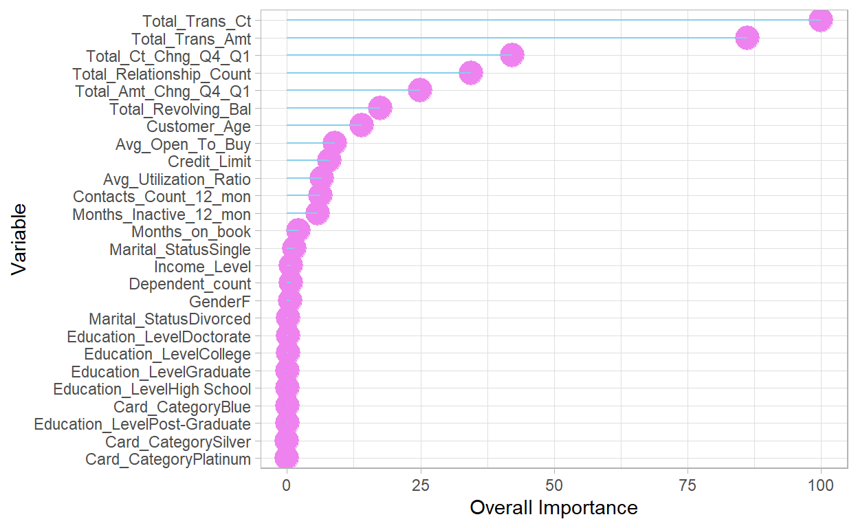
v. Gradient Boosting Tree Total NA
Original data set with Total Missing Value Replaced
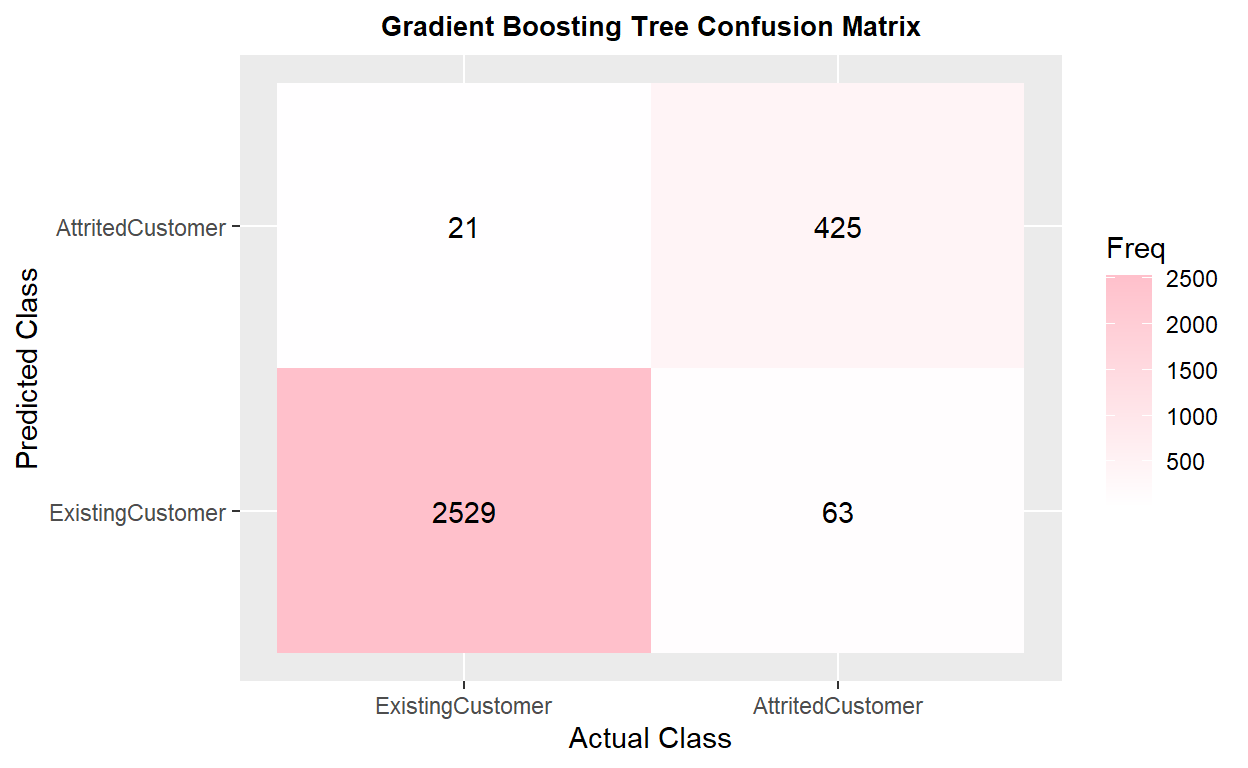
The model has 0.9681 of accuracy and 0.8781 in kappa. The recall is 0.8648 Gradient boosting tree has a better performance compared to the random forest under the same condition.
Show code
# data split
index <- createDataPartition(BankChurners2$Attrition_Flag,
p = .7, list = FALSE, times = 1)
train <- BankChurners2[index,]
test <- BankChurners2[-index,]
# train4
churn_GBM1 <- train(
form = factor(Attrition_Flag) ~.,
data = train,
trControl = trainControl(method = "cv",
number = 10,
classProbs = TRUE),
method = "gbm",
tuneLength = 10,
verbose = FALSE
)
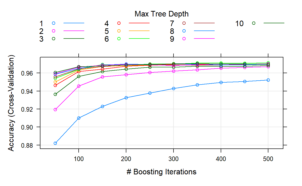
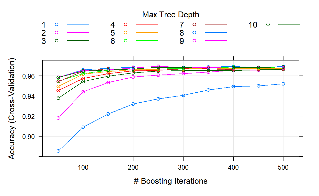
kable(churn_GBM1$bestTune)
| n.trees | interaction.depth | shrinkage | n.minobsinnode | |
|---|---|---|---|---|
| 60 | 500 | 6 | 0.1 | 10 |
Show code
plot(churn_GBM1)
Show code
# test4
churn_GBM_pred1 <- predict(churn_GBM1, test, type = "prob")
churn_GBM_test_pred1 <- cbind(churn_GBM_pred1, test)
churn_GBM_test_pred1 <- churn_GBM_test_pred1 %>%
  mutate(prediction = if_else(AttritedCustomer > ExistingCustomer,
                              "AttritedCustomer", "ExistingCustomer"))
table(churn_GBM_test_pred1$prediction)
AttritedCustomer ExistingCustomer
             446             2592
Show code
# result4
churn_matrix4 <- confusionMatrix(factor(churn_GBM_test_pred1$prediction),
                                 factor(churn_GBM_test_pred1$Attrition_Flag),
                                 positive = "AttritedCustomer")
churn_matrix4
Confusion Matrix and Statistics

                  Reference
Prediction         ExistingCustomer AttritedCustomer
  ExistingCustomer             2529               63
  AttritedCustomer               21              425

               Accuracy : 0.9724
                 95% CI : (0.9659, 0.9779)
    No Information Rate : 0.8394
    P-Value [Acc > NIR] : < 2.2e-16

                  Kappa : 0.8938

 Mcnemar's Test P-Value : 7.696e-06

            Sensitivity : 0.8709
            Specificity : 0.9918
         Pos Pred Value : 0.9529
         Neg Pred Value : 0.9757
             Prevalence : 0.1606
         Detection Rate : 0.1399
   Detection Prevalence : 0.1468
      Balanced Accuracy : 0.9313

       'Positive' Class : AttritedCustomer
Show code
ggplot(as.data.frame(churn_matrix4$table)) +
  geom_raster(aes(x = Reference, y = Prediction, fill = Freq)) +
  geom_text(aes(x = Reference, y = Prediction, label = Freq)) +
  scale_fill_gradient2(low = "darkred", high = "pink",
                       na.value = "grey", name = "Freq") +
  scale_x_discrete(name = "Actual Class") +
  scale_y_discrete(name = "Predicted Class") +
  ggtitle("Gradient Boosting Tree Confusion Matrix") +
  theme(plot.title = element_text(hjust = .5, size = 10, face = "bold"))
Show code
| Overall | |
|---|---|
| Total_Trans_Ct | 100.00000 |
| Total_Trans_Amt | 86.21584 |
| Total_Ct_Chng_Q4_Q1 | 42.17720 |
| Total_Relationship_Count | 34.47348 |
| Total_Amt_Chng_Q4_Q1 | 24.89156 |
| Total_Revolving_Bal | 17.50240 |
Show code
ggplot(var_imp4, aes(x = reorder(rownames(var_imp4), Overall), y = Overall)) +
  geom_point(color = "violet", size = 6, alpha = 1) +
  geom_segment(aes(x = rownames(var_imp4), xend = rownames(var_imp4),
                   y = 0, yend = Overall), color = "skyblue") +
  xlab("Variable") +
  ylab("Overall Importance") +
  theme_light() +
  coord_flip()
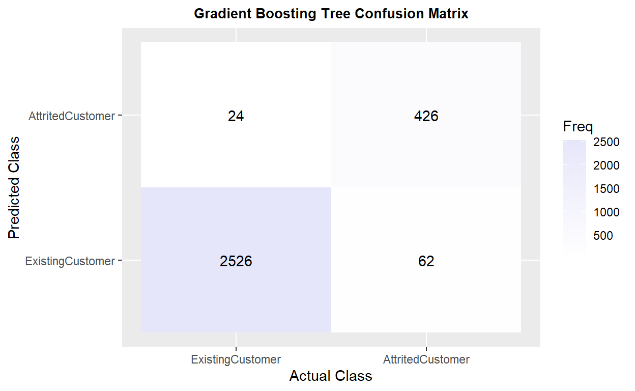
vi. Gradient Boosting Tree Train NA✨
Original data set with Training Set Missing Value Replaced and only replaced missing values in the training set
The model has 0.9691 of accuracy and 0.8805 in kappa, and recall is 0.8545
Show code
# data split
index2 <- createDataPartition(BankChurners1$Attrition_Flag,
                              p = .7, list = FALSE, times = 1)
 train2 <- BankChurners1[index,]
 test2 <- BankChurners1[-index,]
 table(is.na(train2))
 FALSE   TRUE
134991   6789
Show code
# replace missing values in the training set
train2 <- VIM::kNN(train2,
               variable = c("Dependent_count", "Education_Level",
                           "Marital_Status", "Income_Level",
                           "Months_Inactive_12_mon", "Contacts_Count_12_mon",
                           "Total_Revolving_Bal", "Total_Amt_Chng_Q4_Q1",
                           "Total_Ct_Chng_Q4_Q1", "Avg_Utilization_Ratio"),
              k = 10)
# summary(train2)
train2 <- train2[,-c(21:30)]
table(is.na(train2))
 FALSE
141780
Show code
# train5
churn_GBM2 <- train(
  form = factor(Attrition_Flag) ~.,
  data = train2,
  trControl = trainControl(method = "cv",
                           number = 10,
                           classProbs = TRUE),
  method = "gbm",
  tuneLength = 10,
  verbose = FALSE
)
# churn_GBM2
kable(churn_GBM2$bestTune)
| n.trees | interaction.depth | shrinkage | n.minobsinnode | |
|---|---|---|---|---|
| 85 | 250 | 9 | 0.1 | 10 |
Show code
plot(churn_GBM2)
Show code
# test5
churn_GBM_pred2 <- predict(churn_GBM2, test, type = "prob")
churn_GBM_test_pred2 <- cbind(churn_GBM_pred2, test2)
churn_GBM_test_pred2 <- churn_GBM_test_pred2 %>%
  mutate(prediction = if_else(AttritedCustomer > ExistingCustomer,
                              "AttritedCustomer", "ExistingCustomer"))
table(churn_GBM_test_pred2$prediction)
AttritedCustomer ExistingCustomer
             450             2588
Show code
# result5
churn_matrix5 <- confusionMatrix(factor(churn_GBM_test_pred2$prediction),
                                 factor(churn_GBM_test_pred2$Attrition_Flag),
                                 positive = "AttritedCustomer")
churn_matrix5
Confusion Matrix and Statistics

                  Reference
Prediction         ExistingCustomer AttritedCustomer
  ExistingCustomer             2526               62
  AttritedCustomer               24              426

               Accuracy : 0.9717
                 95% CI : (0.9652, 0.9773)
    No Information Rate : 0.8394
    P-Value [Acc > NIR] : < 2.2e-16

                  Kappa : 0.8916

 Mcnemar's Test P-Value : 6.613e-05

            Sensitivity : 0.8730
            Specificity : 0.9906
         Pos Pred Value : 0.9467
         Neg Pred Value : 0.9760
             Prevalence : 0.1606
         Detection Rate : 0.1402
   Detection Prevalence : 0.1481
      Balanced Accuracy : 0.9318

       'Positive' Class : AttritedCustomer
Show code
ggplot(as.data.frame(churn_matrix5$table)) +
  geom_raster(aes(x = Reference, y = Prediction, fill = Freq)) +
  geom_text(aes(x = Reference, y = Prediction, label = Freq)) +
  scale_fill_gradient2(low = "darkred", high = "lavender",
                       na.value = "grey", name = "Freq") +
  scale_x_discrete(name = "Actual Class") +
  scale_y_discrete(name = "Predicted Class") +
  ggtitle("Gradient Boosting Tree Confusion Matrix") +
  theme(plot.title = element_text(hjust = .5, size = 10, face = "bold"))
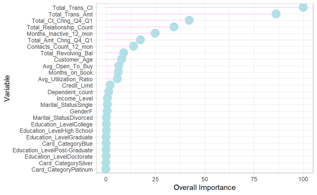
vii. Gradient Boosting Tree Total NA & SMOTE
Original data set with Total Missing Value Replaced and Resampling in the Training Set
The model has 0.9635 of accuracy and 0.8668 in kappa, which is similar to the previous result. The recall is 0.9078 🎉 (Mcnemar’s Test P-Value : 0.02545 🅿)
Show code
# data split
index <- createDataPartition(BankChurners2$Attrition_Flag,
                             p = .7, list = FALSE, times = 1)
train <- BankChurners2[index,]
test <- BankChurners2[-index,]

# train6
churn_GBM3 <- train(
  form = factor(Attrition_Flag) ~.,
  data = train,
  trControl = trainControl(method = "cv",
                           number = 10,
                           classProbs = TRUE,
                           sampling = "smote"),
  method = "gbm",
  tuneLength = 10,
  verbose = FALSE
)
# kable(churn_GBM3$bestTune)
# plot(churn_GBM3)

# test6
churn_GBM_pred3 <- predict(churn_GBM3, test, type = "prob")
churn_GBM_test_pred3 <- cbind(churn_GBM_pred3, test)
churn_GBM_test_pred3 <- churn_GBM_test_pred3 %>%
  mutate(prediction = if_else(AttritedCustomer > ExistingCustomer,
                              "AttritedCustomer", "ExistingCustomer"))
table(churn_GBM_test_pred3$prediction)
AttritedCustomer ExistingCustomer
             529             2509
Show code
# result6
churn_matrix6 <- confusionMatrix(factor(churn_GBM_test_pred3$prediction),
                                 factor(churn_GBM_test_pred3$Attrition_Flag),
                                 positive = "AttritedCustomer")
churn_matrix6
Confusion Matrix and Statistics

                  Reference
Prediction         ExistingCustomer AttritedCustomer
  ExistingCustomer             2472               37
  AttritedCustomer               78              451

               Accuracy : 0.9621
                 95% CI : (0.9547, 0.9686)
    No Information Rate : 0.8394
    P-Value [Acc > NIR] : < 2.2e-16

                  Kappa : 0.8642

 Mcnemar's Test P-Value : 0.0001915

            Sensitivity : 0.9242
            Specificity : 0.9694
         Pos Pred Value : 0.8526
         Neg Pred Value : 0.9853
             Prevalence : 0.1606
         Detection Rate : 0.1485
   Detection Prevalence : 0.1741
      Balanced Accuracy : 0.9468

       'Positive' Class : AttritedCustomer
Show code
ggplot(as.data.frame(churn_matrix6$table)) +
  geom_raster(aes(x = Reference, y = Prediction, fill = Freq)) +
  geom_text(aes(x = Reference, y = Prediction, label = Freq)) +
  scale_fill_gradient2(low = "darkred", high = "firebrick",
                       na.value = "grey", name = "Freq") +
  scale_x_discrete(name = "Actual Class") +
  scale_y_discrete(name = "Predicted Class") +
  ggtitle("Gradient Boosting Tree & SMOTE Confusion Matrix") +
  theme(plot.title = element_text(hjust = .5, size = 10, face = "bold"))

Show code
| Overall | |
|---|---|
| Total_Trans_Ct | 100.000000 |
| Total_Trans_Amt | 30.220501 |
| Total_Ct_Chng_Q4_Q1 | 22.463371 |
| Total_Relationship_Count | 16.367709 |
| Months_Inactive_12_mon | 15.729941 |
| Total_Amt_Chng_Q4_Q1 | 6.665217 |
Show code
ggplot(var_imp4, aes(x = reorder(rownames(var_imp5), Overall), y = Overall)) +
  geom_point(color = "powderblue", size = 6, alpha = 1) +
  geom_segment(aes(x = rownames(var_imp5), xend = rownames(var_imp5),
                   y = 0, yend = Overall), color = "plum1") +
  xlab("Variable") +
  ylab("Overall Importance") +
  theme_light() +
  coord_flip()
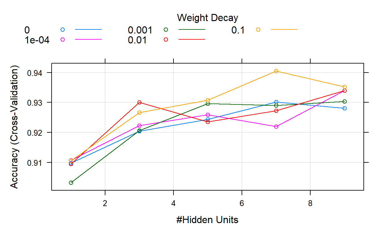
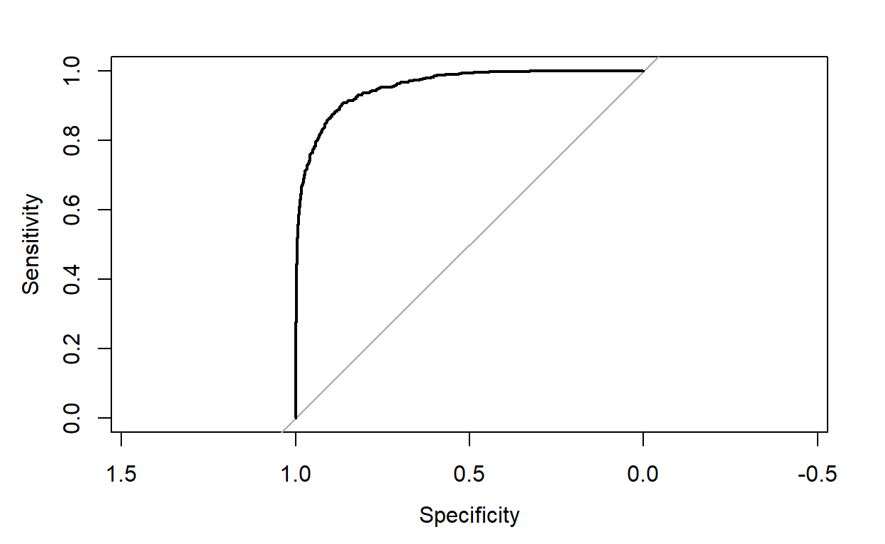
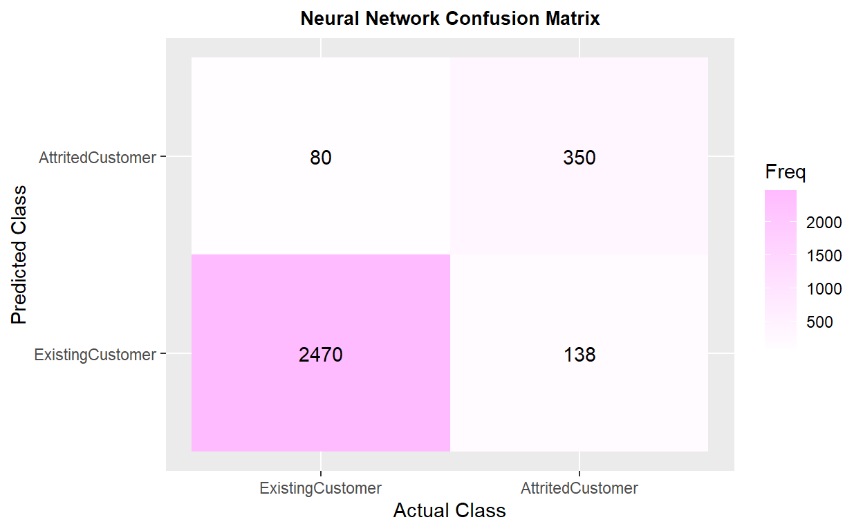
viii. 🌜Neural Network Total NA🕊️
Original data set with Total Missing Value Replaced
The model has 0.9351 of accuracy and 0.7446 in kappa, and recall is 0.7277😕. The ROC curve looks great🏄 ROC result description: _____.
Show code
# train7
churn_NNET <- train(
  form = factor(Attrition_Flag) ~.,
  data = train,
  trControl = trainControl(method = "cv",
                           number = 10,
                           classProb =TRUE),
  method = "nnet",
  preProcess = c("center", "scale"),
  tuneLength = 5,
  trace= FALSE
)
plot(churn_NNET)
Show code
# test7
churn_NNET_pred <- predict(churn_NNET, test, type = "prob")
churn_NNET_test_pred <- cbind(churn_NNET_pred, test)
churn_NNET_test_pred <- churn_NNET_test_pred %>%
  mutate(prediction = if_else(AttritedCustomer > ExistingCustomer,
                              "AttritedCustomer", "ExistingCustomer"))
table(churn_NNET_test_pred$prediction)
AttritedCustomer ExistingCustomer
             430             2608
Show code
Show code
# result7
churn_matrix7 <- confusionMatrix(factor(churn_NNET_test_pred$prediction),
                                 factor(churn_NNET_test_pred$Attrition_Flag),
                                 positive = "AttritedCustomer")
churn_matrix7
Confusion Matrix and Statistics

                  Reference
Prediction         ExistingCustomer AttritedCustomer
  ExistingCustomer             2470              138
  AttritedCustomer               80              350

               Accuracy : 0.9282
                 95% CI : (0.9185, 0.9372)
    No Information Rate : 0.8394
    P-Value [Acc > NIR] : < 2.2e-16

                  Kappa : 0.7205

 Mcnemar's Test P-Value : 0.0001131

            Sensitivity : 0.7172
            Specificity : 0.9686
         Pos Pred Value : 0.8140
         Neg Pred Value : 0.9471
             Prevalence : 0.1606
         Detection Rate : 0.1152
   Detection Prevalence : 0.1415
      Balanced Accuracy : 0.8429

       'Positive' Class : AttritedCustomer
Show code
ggplot(as.data.frame(churn_matrix7$table)) +
  geom_raster(aes(x = Reference, y = Prediction, fill = Freq)) +
  geom_text(aes(x = Reference, y = Prediction, label = Freq)) +
  scale_fill_gradient2(low = "darkred", high = "plum1",
                       na.value = "grey", name = "Freq") +
  scale_x_discrete(name = "Actual Class") +
  scale_y_discrete(name = "Predicted Class") +
  ggtitle("Neural Network Confusion Matrix") +
  theme(plot.title = element_text(hjust = .5, size = 10, face = "bold"))
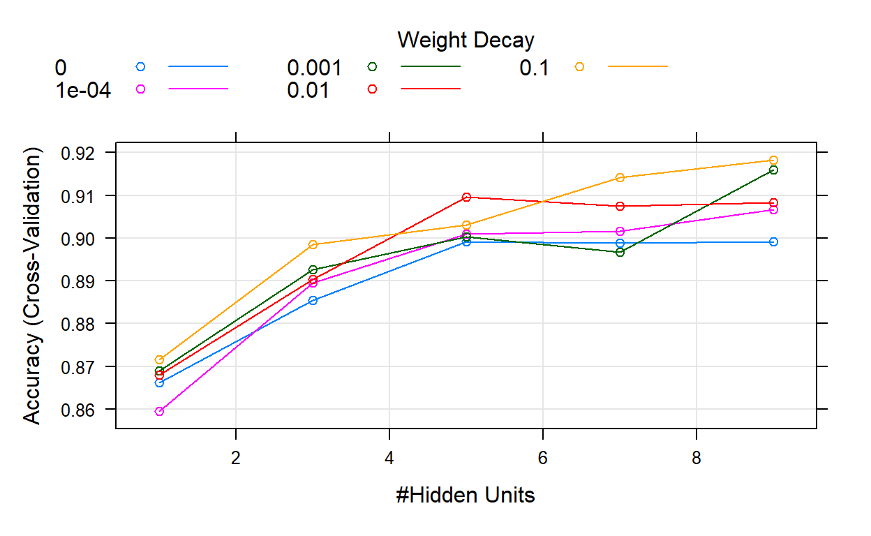
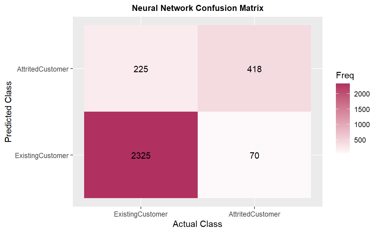
ix. Neural Network Total NA & SMOTE
Original data set with total missing value replaced & SMOTE resampling
The model has _____ of accuracy and _____ in kappa, which is ______ to the previous model. The recall is _____, _____ compared to the prior model.
ROC result description: _____.
Show code
# train8
churn_NNET2 <- train(
  form = factor(Attrition_Flag) ~.,
  data = train,
  trControl = trainControl(method = "cv",
                           number = 10,
                           classProb = TRUE,
                           sampling = "smote"),
  method = "nnet",
  preProcess = c("center", "scale"),
  tuneLength = 5,
  trace= FALSE
)
plot(churn_NNET2)
Show code
# test8
churn_NNET_pred2 <- predict(churn_NNET2, test, type = "prob")
churn_NNET_test_pred2 <- cbind(churn_NNET_pred2, test)
churn_NNET_test_pred2 <- churn_NNET_test_pred2 %>%
  mutate(prediction = if_else(AttritedCustomer > ExistingCustomer,
                              "AttritedCustomer", "ExistingCustomer"))
table(churn_NNET_test_pred2$prediction)
AttritedCustomer ExistingCustomer
             643             2395
Show code
Error in h(simpleError(msg, call)): error in evaluating the argument 'x' in selecting a method for function 'plot': object 'roc_NNET2' not foundShow code
# result8
churn_matrix8 <- confusionMatrix(factor(churn_NNET_test_pred2$prediction),
                                 factor(churn_NNET_test_pred2$Attrition_Flag),
                                 positive = "AttritedCustomer")
churn_matrix8
Confusion Matrix and Statistics

                  Reference
Prediction         ExistingCustomer AttritedCustomer
  ExistingCustomer             2325               70
  AttritedCustomer              225              418

               Accuracy : 0.9029
                 95% CI : (0.8918, 0.9132)
    No Information Rate : 0.8394
    P-Value [Acc > NIR] : < 2.2e-16

                  Kappa : 0.6809

 Mcnemar's Test P-Value : < 2.2e-16

            Sensitivity : 0.8566
            Specificity : 0.9118
         Pos Pred Value : 0.6501
         Neg Pred Value : 0.9708
             Prevalence : 0.1606
         Detection Rate : 0.1376
   Detection Prevalence : 0.2117
      Balanced Accuracy : 0.8842

       'Positive' Class : AttritedCustomer
Show code
ggplot(as.data.frame(churn_matrix8$table)) +
  geom_raster(aes(x = Reference, y = Prediction, fill = Freq)) +
  geom_text(aes(x = Reference, y = Prediction, label = Freq)) +
  scale_fill_gradient2(low = "darkred", high = "maroon",
                       na.value = "grey", name = "Freq") +
  scale_x_discrete(name = "Actual Class") +
  scale_y_discrete(name = "Predicted Class") +
  ggtitle("Neural Network Confusion Matrix") +
  theme(plot.title = element_text(hjust = .5, size = 10, face = "bold"))
VI. Result
Overall, 🌳random forest model has the best performance🏆 compared to gradient boosting tree and neural network🌲, especially after replacing total missing values and using SMOTE to fix 🔧 the imbalanced data set issue. (iv.RF TOTAL NA & SMOTE)
Show code
comparison <- matrix(c(0.9661, 0.8683, 0.8381, 0.9585, 0.8409, 0.8308, 0.9575, 0.8341,
                       0.8062, 0.9549, 0.8423, 0.9344, 0.9681, 0.8781, 0.8648, 0.9691,
                       0.8805, 0.8545, 0.9635, 0.8668, 0.9078, 0.9351, 0.7446, 0.7277,
                       0.0000, 0.0000, 0.0000),
                     ncol = 3, byrow = TRUE)
colnames(comparison) <- c("Accuracy", "Kappa", "Recall")
rownames(comparison) <- c("i.RF TOTAL NA", "ii.RF TOTAL NA & VAR", "iii.RF TRAIN NA",
                          "iv.RF TOTAL NA & SMOTE", "v.GBT TOTAL NA", "vi.GBT TRAIN NA",
                          "vii.GBT TOTAL NA & SMOTE", "viii.NNET TOTAL NA", "ix.NNET TOTAL NA & SMOTE")
comparison <- as.data.frame.matrix(comparison)
kable(comparison) %>%
  row_spec(4, color = "white", background = "#bdaeea")
| Accuracy | Kappa | Recall | |
|---|---|---|---|
| i.RF TOTAL NA | 0.9661 | 0.8683 | 0.8381 |
| ii.RF TOTAL NA & VAR | 0.9585 | 0.8409 | 0.8308 |
| iii.RF TRAIN NA | 0.9575 | 0.8341 | 0.8062 |
| iv.RF TOTAL NA & SMOTE | 0.9549 | 0.8423 | 0.9344 |
| v.GBT TOTAL NA | 0.9681 | 0.8781 | 0.8648 |
| vi.GBT TRAIN NA | 0.9691 | 0.8805 | 0.8545 |
| vii.GBT TOTAL NA & SMOTE | 0.9635 | 0.8668 | 0.9078 |
| viii.NNET TOTAL NA | 0.9351 | 0.7446 | 0.7277 |
| ix.NNET TOTAL NA & SMOTE | 0.0000 | 0.0000 | 0.0000 |
The original model from Kaggle has 0.62 for recall, so 🤠my models did improve the performance of predicting churned customers🥳. They can help companies to identify potential customer churn with higher success rate. The neural network model _____. Based on the variable importance rates, customers’ transaction numbers and amounts, changes in transaction amount, and total product held by customers are the most important⭐ predicting variables in those models. The demographic factors are not important in those models though.
Limitations: