I. The Model
👩💻A Support Vector Machine (SVM) model is a supervised👀 machine learning model used for classification. It is simple but very useful. It uses a tool🔨 called hyperplane to separate data into different groups. It has different methods for both linear and non-linear data. And the methods that are used here are svmLinear and svmPloy.
II. The Process and Results
Since SVM is a supervised model, the first step is to split the dataset into training and testing sets and assume the dataset is clean♻️. After the dataset split, we run🏃 the SVM in the training set and use the trained data to predict the testing set. Finally, we use a 📐📏confusion matrix to show how well is our prediction in terms of accuracy, recall, Specificity, etc.
We are 🔭interested in the effect of data split ratios on the model performance, so we compare two new ratios, 75:25 and 50:50 with the original ratio of 60:40 conducted by Dr.Hunt. We also implement both linear and poly methods on the dataset to see the difference in their performance.
The result for both splits and poly method are better📈 than the original model performance, which means that data split does have an impact on the model fitness. 🎊Because we know that two classes of variables have some overlaps, so it is expected that poly will be a better fit for the dataset. However, we did not test statistical significance for those changes🙊.
Show code
comparison <- matrix(c(0.9333, 0.9000, 0.7938, 0.8500, 0.9444, 0.9167, 0.8333, 1.0000,
                       0.9467, 0.9200, 0.9600, 0.8800, 0.9667, 0.9500, 0.9000, 1.0000),
                    ncol = 4, byrow = TRUE)
colnames(comparison) <- c("Accuracy", "Kappa", "Recall-Versi", "Recall-Virgi")
rownames(comparison) <- c("Linear 60:40", "Linear 75:25", "Linear 50:50", "NonLin 60:40")
comparison <- as.data.frame.matrix(comparison)
kable(comparison)
| Accuracy | Kappa | Recall-Versi | Recall-Virgi | |
|---|---|---|---|---|
| Linear 60:40 | 0.9333 | 0.9000 | 0.7938 | 0.85 |
| Linear 75:25 | 0.9444 | 0.9167 | 0.8333 | 1.00 |
| Linear 50:50 | 0.9467 | 0.9200 | 0.9600 | 0.88 |
| NonLin 60:40 | 0.9667 | 0.9500 | 0.9000 | 1.00 |
III. Application
The SVM model can be used for identifying abnormalities such as fraudulent transactions, material misstatements, bankruptcies, abnormal reserves, etc. Auditors can utilize this machine learning model with other algorithms as well as financial ratios to improve their accuracy and efficiency.
IV. Code
i. Data Split 75:25
Accuracy and Kappa both increased a little✨ bit
Data Preparation
Show code
# data split
iris1 <- iris
train_index <- createDataPartition(iris1$Species, p = .75, list = FALSE, times = 1)

iris_train <- iris1[train_index,]
iris_test <- iris1[-train_index,]
Model
Show code
# train
iris_svm_train <- train(
  form = factor(Species) ~.,
  data = iris_train,
  trControl = trainControl(method = "cv",
                           number = 10,
                           classProbs = TRUE),
  method = "svmLinear",
  preProcess = c("center", "scale"),
  tuneLength = 10
)
# iris_svm_train
summary(iris_svm_train)
Length  Class   Mode
     1   ksvm     S4
Show code
# predict
iris_svm_predict <- predict(iris_svm_train, iris_test, type = "prob")

iris_svm_predict <- cbind(iris_svm_predict, iris_test)
iris_svm_predict <- iris_svm_predict %>%
  mutate(prediction = if_else(setosa > versicolor & setosa > virginica, "setosa",
                              if_else(versicolor > setosa & versicolor > virginica, "versicolor",
                                      if_else(virginica > setosa & virginica > versicolor, "virginica", "PROBLEM"))))
# table(iris_svm_predict$prediction)
confusionMatrix(factor(iris_svm_predict$prediction), factor(iris_svm_predict$Species))
Confusion Matrix and Statistics

            Reference
Prediction   setosa versicolor virginica
  setosa         12          0         0
  versicolor      0         10         0
  virginica       0          2        12

Overall Statistics

               Accuracy : 0.9444
                 95% CI : (0.8134, 0.9932)
    No Information Rate : 0.3333
    P-Value [Acc > NIR] : 1.728e-14

                  Kappa : 0.9167

 Mcnemar's Test P-Value : NA

Statistics by Class:

                     Class: setosa Class: versicolor Class: virginica
Sensitivity                 1.0000            0.8333           1.0000
Specificity                 1.0000            1.0000           0.9167
Pos Pred Value              1.0000            1.0000           0.8571
Neg Pred Value              1.0000            0.9231           1.0000
Prevalence                  0.3333            0.3333           0.3333
Detection Rate              0.3333            0.2778           0.3333
Detection Prevalence        0.3333            0.2778           0.3889
Balanced Accuracy           1.0000            0.9167           0.9583
Plot SVM
Show code
sv1 <- iris_train[iris_svm_train$finalModel@SVindex,]
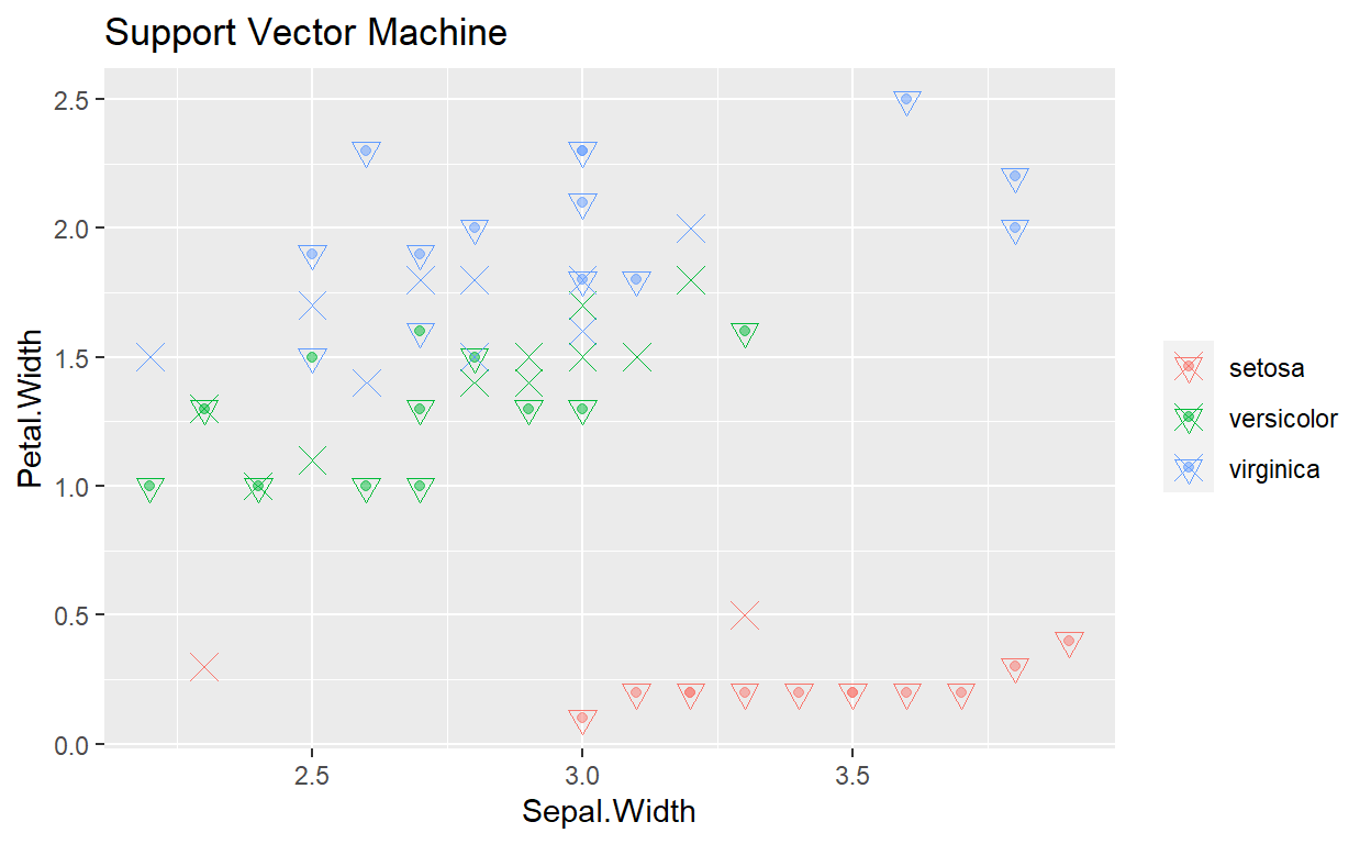
ggplot(data = iris_test, mapping = aes(x = Sepal.Width, y= Petal.Width, color = Species)) +
geom_point(alpha = .5) +
geom_point(data = iris_svm_predict, mapping = aes(x = Sepal.Width, y = Petal.Width, color = prediction),
shape = 6, size = 3) +
geom_point(data = sv1, mapping = aes(x = Sepal.Width, y = Petal.Width), shape = 4, size = 4) +
theme(legend.title = element_blank()) +
ggtitle("Support Vector Machine")
ii. Data Split 50:50
Accuracy and Kappa both increased a little. Versicolor’s recall increased a lot👏
Model
Show code
# data split
train_index <- createDataPartition(iris1$Species, p = .5, list = FALSE, times = 1)

iris_train <- iris1[train_index,]
iris_test <- iris1[-train_index,]

# train
iris_svm_train <- train(
  form = factor(Species) ~.,
  data = iris_train,
  trControl = trainControl(method = "cv",
                           number = 10,
                           classProbs = TRUE),
  method = "svmLinear",
  preProcess = c("center", "scale"),
  tuneLength = 10
)
# iris_svm_train
summary(iris_svm_train)
Length  Class   Mode
     1   ksvm     S4
Show code
# predict
iris_svm_predict <- predict(iris_svm_train, iris_test, type = "prob")

iris_svm_predict <- cbind(iris_svm_predict, iris_test)
iris_svm_predict <- iris_svm_predict %>%
  mutate(prediction = if_else(setosa > versicolor & setosa > virginica, "setosa",
                              if_else(versicolor > setosa & versicolor > virginica, "versicolor",
                                      if_else(virginica > setosa & virginica > versicolor, "virginica", "PROBLEM"))))
# table(iris_svm_predict$prediction)
confusionMatrix(factor(iris_svm_predict$prediction), factor(iris_test$Species))
Confusion Matrix and Statistics

            Reference
Prediction   setosa versicolor virginica
  setosa         25          0         0
  versicolor      0         24         3
  virginica       0          1        22

Overall Statistics

               Accuracy : 0.9467
                 95% CI : (0.869, 0.9853)
    No Information Rate : 0.3333
    P-Value [Acc > NIR] : < 2.2e-16

                  Kappa : 0.92

 Mcnemar's Test P-Value : NA

Statistics by Class:

                     Class: setosa Class: versicolor Class: virginica
Sensitivity                 1.0000            0.9600           0.8800
Specificity                 1.0000            0.9400           0.9800
Pos Pred Value              1.0000            0.8889           0.9565
Neg Pred Value              1.0000            0.9792           0.9423
Prevalence                  0.3333            0.3333           0.3333
Detection Rate              0.3333            0.3200           0.2933
Detection Prevalence        0.3333            0.3600           0.3067
Balanced Accuracy           1.0000            0.9500           0.9300
iii. Kernel: svmPoly
Has the 🏆best overall and individual class performance
Model
Show code
train_index <- createDataPartition(iris1$Species, p = .6, list = FALSE, times = 1)

iris_train <- iris1[train_index,]
iris_test <- iris1[-train_index,]

# train
iris_svm_train <- train(
  form = factor(Species) ~.,
  data = iris_train,
  trControl = trainControl(method = "cv",
                           number = 10,
                           classProbs = TRUE),
  method = "svmPoly",
  preProcess = c("center", "scale"),
  tuneLength = 10
)
summary(iris_svm_train)
Length  Class   Mode
     1   ksvm     S4
Show code
# predict
iris_svm_predict <- predict(iris_svm_train, iris_test, type = "prob")
iris_svm_predict <- cbind(iris_svm_predict, iris_test)

iris_svm_predict <- iris_svm_predict %>%
  mutate(prediction = if_else(setosa > versicolor & setosa > virginica, "setosa",
                              if_else(versicolor >setosa & versicolor > virginica, "versicolor",
                                      if_else(virginica > setosa & virginica > versicolor, "virginica", "PROBLEM"))))
# table(iris_svm_predict$prediction)
confusionMatrix(factor(iris_svm_predict$prediction), factor(iris_test$Species))
Confusion Matrix and Statistics

            Reference
Prediction   setosa versicolor virginica
  setosa         20          0         0
  versicolor      0         18         0
  virginica       0          2        20

Overall Statistics

               Accuracy : 0.9667
                 95% CI : (0.8847, 0.9959)
    No Information Rate : 0.3333
    P-Value [Acc > NIR] : < 2.2e-16

                  Kappa : 0.95

 Mcnemar's Test P-Value : NA

Statistics by Class:

                     Class: setosa Class: versicolor Class: virginica
Sensitivity                 1.0000            0.9000           1.0000
Specificity                 1.0000            1.0000           0.9500
Pos Pred Value              1.0000            1.0000           0.9091
Neg Pred Value              1.0000            0.9524           1.0000
Prevalence                  0.3333            0.3333           0.3333
Detection Rate              0.3333            0.3000           0.3333
Detection Prevalence        0.3333            0.3000           0.3667
Balanced Accuracy           1.0000            0.9500           0.9750